Embark on an enlightening journey through the realm of probability with Unit 12 Test Study Guide Probability. This meticulously crafted guide unlocks the fundamental principles of probability, empowering you with the knowledge to navigate complex probability scenarios with confidence.
Delve into the intricacies of probability distributions, conditional probability, and independence, gaining a deep understanding of the role of sample space in probability calculations. Master the binomial, Poisson, geometric, and negative binomial distributions, equipping yourself with the tools to solve real-world probability problems.
Basic Probability Concepts
Probability theory provides a framework for quantifying the likelihood of events occurring. It underpins various fields, including statistics, finance, and machine learning.
Sample Space
The sample space of an experiment is the set of all possible outcomes. For instance, when flipping a coin, the sample space is heads, tails. In rolling a die, the sample space is 1, 2, 3, 4, 5, 6.
Conditional Probability and Independence

In probability theory, conditional probability and independence are fundamental concepts that describe the relationships between events. Conditional probability quantifies the likelihood of an event occurring given that another event has already occurred, while independence indicates that the occurrence of one event does not affect the probability of another.
Conditional Probability
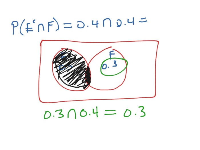
Conditional probability, denoted as P(A|B), represents the probability of event A occurring given that event B has already occurred. It is calculated as the ratio of the probability of the intersection of events A and B to the probability of event B:
P(A|B) = P(A ∩ B) / P(B)
For example, suppose we have a deck of 52 cards and we draw one card. The probability of drawing a heart is 13/52 = 1/4. If we then draw a second card without replacing the first, the probability of drawing another heart given that the first card was a heart is 12/51, since there are now only 12 hearts remaining in the deck of 51 cards.
Independence
Two events A and B are considered independent if the occurrence of one event does not affect the probability of the other event. Mathematically, this means that:
P(A|B) = P(A)
For example, the outcome of a coin flip is independent of the outcome of a die roll. The probability of getting heads on a coin flip is 1/2, regardless of whether the die shows an even or odd number.
Bayes’ Theorem
Bayes’ theorem provides a framework for calculating conditional probabilities when the prior probabilities of events are known. It is expressed as:
P(A|B) = P(B|A)
P(A) / P(B)
Where P(A) is the prior probability of event A, P(B) is the prior probability of event B, P(A|B) is the posterior probability of event A given that event B has occurred, and P(B|A) is the posterior probability of event B given that event A has occurred.
Bayes’ theorem is widely used in various fields, including statistics, machine learning, and medical diagnosis, to update probabilities based on new information.
Discrete Probability Distributions
Discrete probability distributions describe the probability of obtaining specific values for discrete random variables. These distributions are commonly used in various real-world scenarios, such as quality control, epidemiology, and finance.
Binomial Distribution, Unit 12 test study guide probability
The binomial distribution models the number of successes in a sequence of independent experiments, each with a constant probability of success. It is widely used in applications such as quality control, medical testing, and opinion polls.
Formula:P(X = k) = (n! / (k! – (n – k)!)) – p^k – (1 – p)^(n – k)
- n: number of trials
- k: number of successes
- p: probability of success
Poisson Distribution
The Poisson distribution describes the number of events occurring within a fixed interval of time or space, assuming that these events occur independently and at a constant average rate.
Formula:P(X = k) = (e^-λ – λ^k) / k!
- k: number of events
- λ: average rate of events
Geometric Distribution
The geometric distribution models the number of trials required to obtain the first success in a sequence of independent experiments, each with a constant probability of success.
Formula:P(X = k) = (1 – p)^k – p
- k: number of trials
- p: probability of success
Negative Binomial Distribution
The negative binomial distribution generalizes the geometric distribution to model the number of trials required to obtain a specified number of successes in a sequence of independent experiments.
Formula:P(X = k) = (k + r – 1)! / (k! – (r – 1)!) – p^r – (1 – p)^k
- k: number of trials
- r: number of successes
- p: probability of success
Continuous Probability Distributions: Unit 12 Test Study Guide Probability
Continuous probability distributions are used to model random variables that can take on any value within a given interval. They are characterized by their probability density function (PDF), which describes the probability of the random variable taking on a specific value.
Normal Distribution
The normal distribution is a continuous probability distribution that is symmetric and bell-shaped. It is often used to model real-world data that is normally distributed, such as heights, weights, and test scores. The PDF of the normal distribution is given by:“`f(x) = (1 / (σ√(2π)))
e^(-(x-μ)² / (2σ²))
“`where μ is the mean of the distribution and σ is the standard deviation.
Exponential Distribution
The exponential distribution is a continuous probability distribution that is used to model the time between events that occur randomly. It is often used to model the time between failures of equipment or the time between arrivals of customers. The PDF of the exponential distribution is given by:“`f(x) = λ
e^(-λx)
“`where λ is the rate parameter of the distribution.
Gamma Distribution
The gamma distribution is a continuous probability distribution that is used to model the sum of independent exponential random variables. It is often used to model the distribution of waiting times or the distribution of the size of a population.
The PDF of the gamma distribution is given by:“`f(x) = (λ^α / Γ(α))
- x^(α-1)
- e^(-λx)
“`where α is the shape parameter of the distribution and λ is the rate parameter.
Uniform Distribution
The uniform distribution is a continuous probability distribution that is used to model random variables that are equally likely to take on any value within a given interval. It is often used to model the distribution of a random variable that is chosen randomly from a finite set of values.
The PDF of the uniform distribution is given by:“`f(x) = 1 / (b-a)“`where a and b are the lower and upper bounds of the interval, respectively.
Triangular Distribution
The triangular distribution is a continuous probability distribution that is used to model random variables that are more likely to take on values near the center of the distribution than at the extremes. It is often used to model the distribution of a random variable that is estimated from a small sample size.
The PDF of the triangular distribution is given by:“`f(x) = (2 / (b-a))
(x-a) / (b-a)
“`where a and b are the lower and upper bounds of the interval, respectively, and c is the mode of the distribution.
Hypothesis Testing

Hypothesis testing is a statistical method used to determine whether a hypothesis about a population parameter is supported by the available evidence. It involves comparing a null hypothesis, which represents the claim being tested, with an alternative hypothesis, which represents the alternative claim.
The decision to reject or fail to reject the null hypothesis is based on the p-value, which is the probability of observing the sample data if the null hypothesis is true.
Steps Involved in Hypothesis Testing
- State the null and alternative hypotheses.
- Set the significance level.
- Calculate the test statistic.
- Determine the p-value.
- Make a decision about the null hypothesis.
Concepts of Null and Alternative Hypotheses
The null hypothesis (H0) represents the claim that there is no significant difference between the observed data and what would be expected if the null hypothesis were true. The alternative hypothesis (Ha) represents the claim that there is a significant difference between the observed data and what would be expected if the null hypothesis were true.
Using p-Values and Significance Levels in Hypothesis Testing
The p-value is the probability of observing the sample data if the null hypothesis is true. The significance level is the maximum p-value at which the null hypothesis will be rejected. If the p-value is less than the significance level, the null hypothesis is rejected in favor of the alternative hypothesis.
Otherwise, the null hypothesis is not rejected.
Questions and Answers
What is the fundamental principle of probability?
Probability measures the likelihood of an event occurring, ranging from 0 (impossible) to 1 (certain).
How is conditional probability used?
Conditional probability calculates the likelihood of an event occurring given that another event has already occurred.
What is the significance of hypothesis testing?
Hypothesis testing provides a framework for evaluating the validity of claims about a population based on sample data.